Hello! welcome once again to the continuation of the last blog post about audio analysis using the Librosa python library, if you missed this article don't worry here you can enjoy audio analysis techniques with Librosa.

The Concept of Audio

Audio is a sound, especially when recorded, transmitted, or reproduced. Also, we can say Audio is the physical representation of sound and its frequency ranges from 20HZ to 20 Kilohertz, which limits the human hearing range. Frequencies below 20Hz and above 20KHz are inaudible for humans because they are either low or too high. This can be represented by taking the sample rate 16kHz,44.1kHZ, ...

The sample rate is the number of samples taken per second, When we mention that audio has a 44-kilohertz sample rate, It means we take 44000 samples or measurements per second. The more samples you get the high the quality of sound you can capture. These samples over time result in a Waveform.

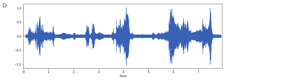
Waveform Image

The presentation of the waveform on the Y-axis is an Amplitude and on the X-axis is time. Machine learning techniques can be applied to waveforms but before that let’s understand on features of the waveform which are called Spectrogram.

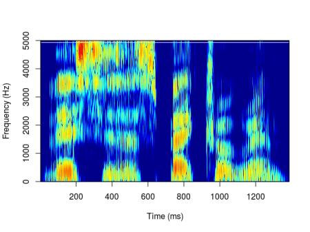
Spectrogram Image

Spectrogram - is the visual representation of all the frequencies over time which is derived from waveform audio format. The Y-axis is the frequency in hertz, the X-axis is the time and the color represents the magnitude or amplitude. The brighter the higher it is usually in decibels(unit of measure).

We can convert the waveform to a spectrogram, which is technically equivalent to an image. Researchers have found that we can effectively apply computer vision techniques to the spectrogram. It turns out that we can classify sound with the same techniques used to classify images. With spectrogram, the machine learning techniques/models can extract the dominant audio per timeframe by finding patterns in the spectrogram.

Applying ML on Audio

For performing audio classification you can go with one of these two options:

1. Use a pre-trained model by updating layers depending on the problem on hand.
2. The second option is to train your own model using machine learning frameworks like Tensorflow and Pytorch.

We will be implementing audio classification using the Tensorflow machine learning framework, considering the raw audio dataset that we will categorize into cat and dog audios. As always done in machine learning raw data need to be preprocessed into another form then followed by training of the final solution. So here we are going to work with datasets from Kaggle which contain audios of dogs and cats. We will pre-process the audio followed by building and training a deep learning model to perform classification with Tensorflow. At the end, we will test our final model with new audios with both cats and dogs to see how it will perform classification.

Before anything, we should import the libraries that we will be using for data preprocessing and building an audio classification model.

# import library
import librosa
import pandas as pd
import numpy as np
import seaborn as sns
import matplotlib.pyplot as plt

import tensorflow as tf
from tensorflow.keras.layers.experimental import preprocessing
from tensorflow.keras.preprocessing.image import load_img, img_to_array
from tensorflow.keras.models import Sequential
from tensorflow.keras.layers import Dense, Dropout, Flatten, Conv2D, MaxPool2D, BatchNormalization, Input

Then we should load the datasets ready for analysis

df = pd.read_csv("train_test_split.csv")

# setting train and test path
dog_train_path = "cats_dogs/train/dog/"
dog_test_path = "cats_dogs/test/test/"

cat_train_path = "cats_dogs/train/cat/"
cat_test_path = "cats_dogs/test/cats/"

But we should work on assigning labels to the train and test path we have specified on the above code.

# assigning lables to train and test files
test_cat = df[['test_cat']].dropna().rename(index=str, columns={"test_cat": "file"}).assign(label=0)
test_dog = df[['test_dog']].dropna().rename(index=str, columns={"test_dog": "file"}).assign(label=1)
train_cat = df[['train_cat']].dropna().rename(index=str, columns={"train_cat": "file"}).assign(label=0)
train_dog = df[['train_dog']].dropna().rename(index=str, columns={"train_dog": "file"}).assign(label=1)

test_df = pd.concat([test_cat, test_dog]).reset_index(drop=True)
train_df = pd.concat([train_cat, train_dog]).reset_index(drop=True)

The next step is to create a validation set from the train data file for model validation during training.

# setting train and test data path
train_dir='cats_dogs/train'
test_dir='cats_dogs/test'

file_train = tf.io.gfile.glob(train_dir + '/*/*')
file_train = tf.random.shuffle(file_train)
train_ds=file_train[:168]
val_ds = file_train[168:168+42]

file_test = tf.io.gfile.glob(test_dir + '/*/*')
file_test = tf.random.shuffle(file_test)
test_ds=file_test

The first task after the analysis of audio data we should convert it into waveform representation.

def get_waveform_label(file):
    lab = tf.strings.split(file, os.path.sep)[-2]
    audio_binary = tf.io.read_file(file)
    audio, _ = tf.audio.decode_wav(audio_binary)
    waveform=tf.squeeze(audio, axis=-1)
    return waveform, lab

AUTO = tf.data.AUTOTUNE
files_ds = tf.data.Dataset.from_tensor_slices(train_ds)
waveform_ds = files_ds.map(get_waveform_label, num_parallel_calls=AUTO)

Then waveform representation should be converted/constructed into spectrogram representation.

def get_spectrogram_label(audio, label):
    padding = tf.zeros([300000]-tf.shape(audio), dtype=tf.float32)
    wave = tf.cast(audio, tf.float32)
    eq_length = tf.concat([wave, padding], 0)
    spectrogram = tf.signal.stft(eq_length, frame_length=210, frame_step=110)
    spectrogram = tf.abs(spectrogram)
    spectrogram = tf.expand_dims(spectrogram, -1)
    label_id = tf.argmax(label == labels)
    return spectrogram, label_id

Then, it's time to apply the get_waveform_label and get_spectrogram_label to the train, validation, and test datasets.

def preprocess(file):
    files_ds = tf.data.Dataset.from_tensor_slices(file)
    output_ds = files_ds.map(get_waveform_label,num_parallel_calls=AUTO)
    output_ds = output_ds.map(get_spectrogram_label,num_parallel_calls=AUTO)
    return output_ds

train_ds = spectrogram_ds
val_ds = preprocess(val_ds)
test_ds = preprocess(test_ds)

batch_size = 64
train_ds = train_ds.batch(batch_size)
val_ds = val_ds.batch(batch_size)

After conversion, the spectrogram representation of cats and dogs can be observed as below.

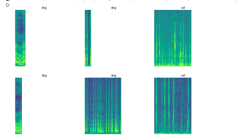
Spectrogram visualization

From, spectrogram form Machine learning can be able to extract patterns and classify the data as expected.

It's time to define our deep learning model using the Tensorflow framework

model = Sequential([
   Input(shape=input_shape), preprocessing.Resizing(32, 32), norm_layer,
   Conv2D(32,3, activation='relu'),
   Conv2D(64,3, activation='relu'),
   MaxPool2D(),
   Dropout(0.5),
   Conv2D(128,7, activation='relu'),
   Conv2D(256,7, activation='relu'),
   MaxPool2D(),
   Dropout(0.5),
   Flatten(),
   Dense(128, activation='relu'),
   Dropout(0.2),
   Dense(16, activation='relu'),
   Dense(num_labels),
])

After defining labels we can compile and print the summary of our model ready for training.

model.compile(optimizer = 'adam', loss = 'binary_crossentropy', metrics = ['accuracy'])
model.summary()

Then it's time to train our model with 20 epochs

his = model.fit(train_ds, epochs=20, validation_data=val_ds)

After training, we should evaluate the model to see how well it is using accuracy evaluation metrics.

test_acc = sum(y_pred == y_true) / len(y_true)
print(f'Test set accuracy: {test_acc:.0%}')

Test set accuracy: 60%

Copy

We get a test accuracy of 60%. Increasing the number of training epochs will increase this accuracy score.

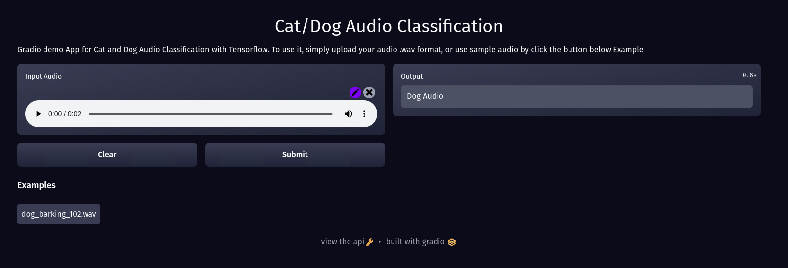
Wow! nice work, hope you have learned something from this article, you can test the model by using the demo application I deployed on Huggingface space using gradio so that you can try to upload the audio file in .wav format to get a prediction.

gradio demo app interface

Point To Note:

You are not limited to using spectrogram for extraction of features from audio data, you can opt to use Mel-Frequency Cepstral Coefficients(MFCCs), Chroma feature, and more depending on the nature of the problem you are trying to solve or you can try to create two different models by using different features like one using spectrograms and another with Mel-Frequency Cepstral Coefficients to see which one can solve the challenge effectively.

Thank you hope this article is useful, keep updated by subscribing to our blog post and don't forget to share with others.

You can access the full codes used for this article here.