Audio Analysis With Librosa

In most cases, data analysis projects are done in tabular data, text data, or image data as the common data available. Tabular data are commonly used to demonstrate the various applications of machine learning simply is easier to work with compared to unstructured data. In today's article, we will be working with the python library Librosa to analyze audio data.

Data analysis varies depending on the nature of the data you are working with each data type has a different technique of preprocessing in machine learning for example on images, it looks on different edges like the human eye and nose, then for the machine to understand should be transformed into numerical features to derive features from the image's pixel values using different filters depending on the application.

What is Audio Analysis

According to Wikipedia, Audio Analysis refers to the extraction of information and meaning from audio signals for analysis, classification, storage, retrieval, synthesis, etc. The observation mediums and interpretation methods vary, as audio analysis can refer to the human ear and how people interpret the audible sound source, or it could refer to using technology such as an Audio analyzer to evaluate other qualities of a sound source such as amplitude, distortion, frequency response, and more. Once an audio source's information has been observed, the information revealed can then be processed for the logical, emotional, descriptive, or otherwise relevant interpretation by the user.

Audios can be presented in different computer-readable formats such as: -

• Wav (Waveform Audio File) format
• WMA (Windows Media Audio) format
• mp3 (MPEG-1 Audio Layer 3) format.

A typical audio processing process involves the extraction of acoustics features relevant to the task at hand, followed by decision-making schemes that involve classification, detection, and knowledge fusion.

Before looking at Librosa, let's understand what are features can be extracted and transformed from audios for machine learning processing.

Some data features and transformations that are important in audio processing are Linear-prediction cepstral coefficients(LFCCs), Bark-frequency cepstral coefficients(BFCCs), Mel-frequency cepstral coefficients(MFCCs), spectrum,cepstrum, spectrogram, Gammatone-frequency cepstral coefficients (GFCCs), and more.

Python has a couple of tools that are used for data extraction and analysis in audios such as Magenta, pyAudioAnalysis, Librosa, and more.

Magenta

Magenta is an open-source Python package built on top of TensorFlow to manipulate image and music data to train a machine learning model with the generative model as the output. To learn more about Magenta here you go.

pyAudioAnalysis

pyAudioAnalysis is a python library covering a wide range of audio analysis tasks. Through pyAudioAnalysis you can perform features extraction and representation from audios, Training, parameter tuning, and evaluation of audio classifiers, classify unknown sounds, detection of audio events, exclude silence periods from long recordings, and more.

To learn more about pyAudioAnalysis here you go.

Finally, let's dive into our today's main topic

Librosa

Librosa is a Python package developed for music and audio analysis. It is specific on capturing the audio information to be transformed into a data block. However, the documentation and example are good to understand how to work with audio data science projects.

Librosa is basically used when we work with audio data like in music generation(using LSTM's), Automatic Speech Recognition. It provides the building blocks necessary to create the music information retrieval systems.

We are going to use Librosa to perform some analysis of audio datasets. Let's set our environment ready for analysis by installing the Librosa python library.

pip install librosa

Once the installation is complete it's time to call Librosa for further analysis, this can be done simply by importing.

import librosa

Then, we want to use librosa for the analysis of audio data so it's time to load the data into a machine to become ready for analysis. The datasets contain dog and cat sounds from kaggle, you can access the dataset from this link

Using Librosaload function we can read the specific audio from dog and cat sounds datasets

# %loading the audio with librosa
data, sampling_rate = librosa.load('cats_dogs/train/cat/cat_125.wav')

The output of the data loader from librosa are two objects, the first is data; a NumPy array of an audio file and the corresponding sampling rate by which it was extracted.

Then, Let's represent this as a waveform by using the librosa.display function

import numpy as np
import matplotlib.pyplot as plt
import librosa.display

plt.figure(figsize=(12, 4))
librosa.display.waveplot(data, sr=sampling_rate)
plt.show()

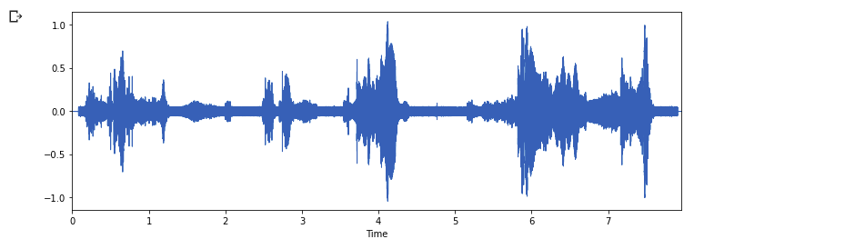
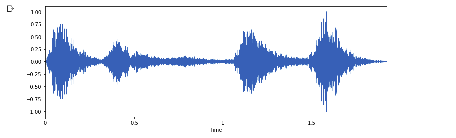
Waveform presentation of cat audio

The same process can be performed for dog sound

# %waveform represenation for dog audio
data, sampling_rate = librosa.load('cats_dogs/train/dog/dog_barking_87.wav')

plt.figure(figsize=(12, 4))
librosa.display.waveplot(data, sr=sampling_rate)
plt.show()

Waveform presentation of dog audio

Nice, we can see the difference between cat audio waveform and dog audio waveform simply by using the librosa.display function. The vertical side represents the Amplitude of the audio and the horizontal axis represents Time taken for the audio at a specific frequency.

Let's try to map the audio from the time domain to the frequency domain using the fast Fourier transform since an audio signal is comprised of several single-frequency sound waves. The aim of using the Fourier transform is to converts the signal from the time domain into the frequency domain. This process will lead us to obtain something called spectrum

Librosa has a function called stft which provides a simple way to plot the transformation of an audio signal to a frequency domain. Some of the important parameters involved are n_fft the length of the windowed signal after padding with zeros, hop_length the frame size, or the size of the Fast Fourier Transform.

n_fft = 2048
plt.figure(figsize=(12, 4))
ft = np.abs(librosa.stft(data[:n_fft], hop_length = n_fft+1))
plt.plot(ft);
plt.title('Spectrum');
plt.xlabel('Frequency Bin');
plt.ylabel('Amplitude');

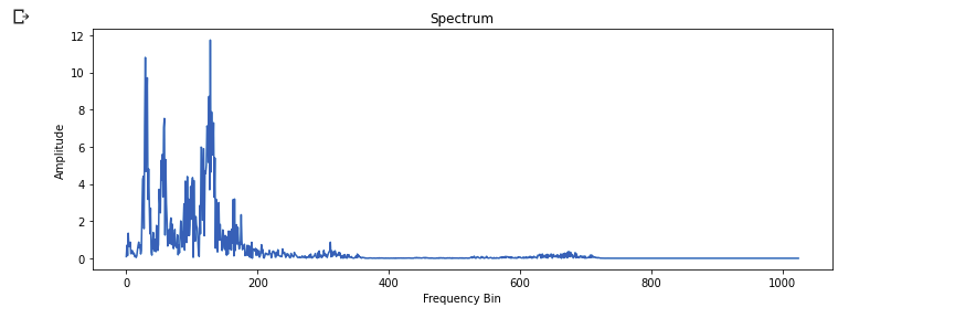
Spectrum using Librosa

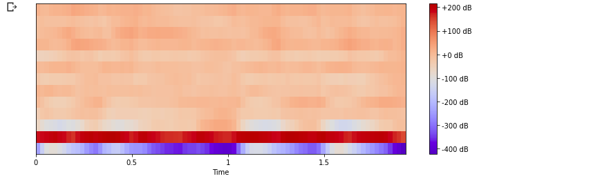
Then, we can opt to look at Time-Frequency Representation which is commonly known as a spectrogram. The spectrogram shows the intensity of frequencies over time. A spectrogram is simply the squared magnitude of the STFT. This gives the representation of time along the x-axis, frequency along the y-axis, and corresponding amplitudes are represented with color. For speech recognition tasks the window used for FFT is 20-30ms as humans can't utter more than one phoneme in this time frame. Windows are overlapped at 50% for it. It can vary between 25% to 75% as per the use case. If s = 16Khz and window duration = 25ms, them samples in window = 16000 25 0.001 = 400 units.If window overlap is 50% then 400*50% = 200 units is the hope for the window. 200 units of frequency bins that represent a B < 16000/2.

n_fft = 2048
S = librosa.amplitude_to_db(abs(ft))
plt.figure(figsize=(12, 4))
librosa.display.specshow(S, sr=sampling_rate, hop_length=512, x_axis='time', y_axis='linear')
plt.colorbar(format='%+2.0f dB')
plt.show()

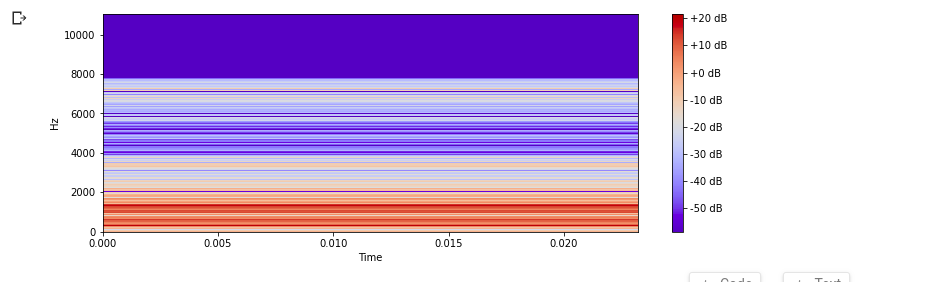
Time-Amplitude Representation using Librosa

Then, we can opt to look at a small set of features usually about 10-20 which concisely describe the overall shape of spectral envelope called Mel Frequency Cepstral Coefficients(MFCCs).

plt.figure(figsize=(12, 4))
mfccs = librosa.feature.mfcc(data, sr=sampling_rate, n_mfcc=13) #computed MFCCs over frames.
librosa.display.specshow(mfccs, sr=sampling_rate, x_axis='time')
plt.colorbar(format='%+2.0f dB')
plt.show()

Mel Frequency Cepstral Coefficients

Further analysis on MFCCs can be done on feature scaling with MinMaxScaler module for data preprocessing.

The best of Librosa offers a couple of audios features function so it depends on the nature of the problem you're solving and which features do you want to look at.

Data Science project is not always about tabular, text, or image data. Sometimes you could use non-conventional data such as audio. In this article, I have demonstrated some audio analysis techniques you can learn more by reading a couple of articles, research, and projects.

Kudos to Leland Roberts for his wonderful article about audio analysis. In the coming articles, we will see how to build an audio classifier model using the same datasets we analyzed in this article, consider subscribing to our blog posts to stay updated.

Thank you you can find the full notebook used in the demonstration here, remember sharing is caring.